
| 일 | 월 | 화 | 수 | 목 | 금 | 토 |
|---|---|---|---|---|---|---|
| 1 | 2 | 3 | 4 | 5 | 6 | |
| 7 | 8 | 9 | 10 | 11 | 12 | 13 |
| 14 | 15 | 16 | 17 | 18 | 19 | 20 |
| 21 | 22 | 23 | 24 | 25 | 26 | 27 |
| 28 | 29 | 30 |
- AI 경진대회
- 편스토랑
- 코로나19
- 더현대서울 맛집
- 맥북
- 편스토랑 우승상품
- PYTHON
- Real or Not? NLP with Disaster Tweets
- 우분투
- 금융문자분석경진대회
- programmers
- 백준
- 파이썬
- ChatGPT
- Docker
- 프로그래머스
- dacon
- leetcode
- 프로그래머스 파이썬
- 자연어처리
- 데이콘
- ubuntu
- Baekjoon
- SW Expert Academy
- Git
- 캐치카페
- hackerrank
- github
- gs25
- Kaggle
- Today
- Total
솜씨좋은장씨
[DACON] 소설 작가 분류 AI 경진대회 5일차! 본문

소설 작가 분류 AI 경진대회
출처 : DACON - Data Science Competition
dacon.io
소설 작가 분류 AI 경진대회 5일차!
요즘 오랜만에 NLP 대회가 열려 퇴근 후가 즐거운 나날입니다.
오늘은 전처리 방법을 바꾸고 베이스라인 코드에있는 모델을 활용하여 결과를 도출해보았습니다.
모든 과정은 aihub에서 지원받은 GPU 환경에서 진행하였습니다.
먼저 첫 번째로 전처리 방식에서 아주 작은 변화를 주었습니다.
먼저 영어 대문자 소문자만 제거해주는 alpha_num 함수에 stopwords에 ' 이 포함되어있는 것들이
alpha_num을 거쳤을때 '이 삭제되지 않아 you've 같은 불용어가 제대로 제외되도록 \' 를 추가했습니다.
def alpha_num(text):
    return re.sub(r"[^A-Za-z0-9\']", ' ', text)
stopwords_list = [ "a", "about", "above", "after", "again", "against", "all", "am", "an", "and", "any", "are", "as",
"at", "be", "because", "been", "before", "being", "below", "between", "both", "but", "by", "could", "will",
"did", "do", "does", "doing", "down", "during", "each", "few", "for", "from", "further", "had", "has",
"have", "having", "he", "he'd", "he'll", "he's", "her", "here", "here's", "hers", "herself", "him", "himself",
"his", "how", "how's", "i", "i'd", "i'll", "i'm", "i've", "if", "in", "into", "is", "it", "it's", "its", "itself",
"let's", "me", "more", "most", "my", "myself", "nor", "of", "on", "once", "only", "or", "other", "ought", "our", "ours",
"ourselves", "out", "over", "own", "same", "she", "she'd", "she'll", "she's", "should", "so", "some", "such", "than", "that",
"that's", "the", "their", "theirs", "them", "themselves", "then", "there", "there's", "these", "they", "they'd", "they'll",
"they're", "they've", "this", "those", "through", "to", "too", "under", "until", "up", "very", "was", "we", "we'd", "we'll",
"we're", "we've", "were", "what", "what's", "when", "when's", "where", "where's", "which", "while", "who", "who's", "whom",
"why", "why's", "with", "would", "you", "you'd", "you'll", "you're", "you've", "your", "yours", "yourself", "yourselves" ]그 다음 baseline코드에서 가져온 불용어 목록을 활용하였습니다.
from tqdm import tqdm
import re
def get_clean_text_list(data_df):
plain_text_list = list(data_df['text'])
clear_text_list = []
for i in tqdm(range(len(plain_text_list))):
plain_text = plain_text_list[i].lower()
plain_text = alpha_num(plain_text)
plain_split = plain_text.split()
plain_split = [word.strip() for word in plain_split if word.strip() not in stopwords_list]
clear_text = " ".join(plain_split).replace("'", "")
clear_text_list.append(clear_text)
return clear_text_list위에서 만든 alpha_num 함수와 baseline 코드에서 가져온 불용어목록을 활용하여
불용어와 특수문자가 제거된 문자열을 만들어주는 함수를 만들었습니다.
train_dataset['clear_text'] = get_clean_text_list(train_dataset)
test_dataset['clear_text'] = get_clean_text_list(test_dataset)이를 활용하여 전처리르 진행하였습니다.
import nltk
from nltk.tokenize import word_tokenize
from nltk.stem.lancaster import LancasterStemmer
stemmer = LancasterStemmer()
import re
X_train = []
train_clear_text = list(train_dataset['clear_text'])
for i in tqdm(range(len(train_clear_text))):
temp = word_tokenize(train_clear_text[i])
temp = [stemmer.stem(word) for word in temp]
temp = [word for word in temp if len(word) > 1]
X_train.append(temp)
X_test = []
test_clear_text = list(test_dataset['clear_text'])
for i in tqdm(range(len(test_clear_text))):
temp = word_tokenize(test_clear_text[i])
temp = [stemmer.stem(word) for word in temp]
temp = [word for word in temp if len(word) > 1]
X_test.append(temp)그리고 이렇게 전처리된 문자열을 다시 nltk를 활용하여 토크나이징 후
LancasterStemmer를 활용하여 어간 추출을 진행하여 나온 단어들 중 길이가 2이상인 토큰들만 남겨 두었습니다.
word_list = []
for i in tqdm(range(len(X_train))):
for j in range(len(X_train[i])):
word_list.append(X_train[i][j])
len(list(set(word_list)))16503이렇게 만든 X_train은 총 몇개의 유니크한 토큰들로 구성되어있는지 확인해보니 16,503개 였습니다.
이 숫자는 Embedding Layer에서 활용합니다.
import numpy as np
y_train = []
labels = list(train_dataset['author'])
for i in tqdm(range(len(labels))):
if labels[i] == 0:
y_train.append([1, 0, 0, 0, 0])
elif labels[i] == 1:
y_train.append([0, 1, 0, 0, 0])
elif labels[i] == 2:
y_train.append([0, 0, 1, 0, 0])
elif labels[i] == 3:
y_train.append([0, 0, 0, 1, 0])
elif labels[i] == 4:
y_train.append([0, 0, 0, 0, 1])
y_train = np.array(y_train)baseline 코드처럼 One-Hot 인코딩을 하지않고 사용해도 되지만 뭔가 습관처럼
저도 모르게 One-Hot 인코딩을 진행하였습니다.
import matplotlib.pyplot as plt
print("최대 길이 :" , max(len(l) for l in X_train))
print("평균 길이 : ", sum(map(len, X_train))/ len(X_train))
plt.hist([len(s) for s in X_train], bins=50)
plt.xlabel('length of Data')
plt.ylabel('number of Data')
plt.show()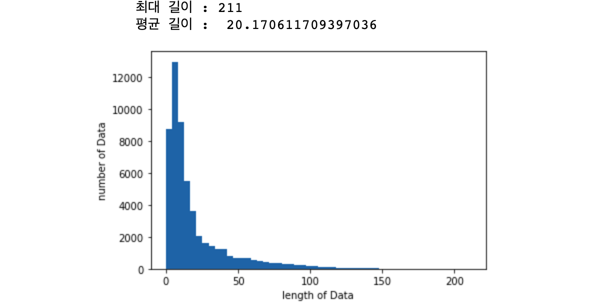
각 데이터 중 가장 긴 데이터는 211, 평균 길이는 20.17입니다.
#파라미터 설정
vocab_size = 16503
embedding_dim = 16
max_len = 211
padding_type='post'
#oov_tok = "<OOV>"위에서 얻은 값들을 바탕으로 파라미터를 설정합니다.
from tensorflow.keras.preprocessing.text import Tokenizer
#tokenizer에 fit
tokenizer = Tokenizer(num_words = vocab_size)#, oov_token=oov_tok)
tokenizer.fit_on_texts(X_train)
word_index = tokenizer.word_index
#데이터를 sequence로 변환해주고 padding 해줍니다.
train_sequences = tokenizer.texts_to_sequences(X_train)
train_padded = pad_sequences(train_sequences, padding=padding_type, maxlen=max_len)
test_sequences = tokenizer.texts_to_sequences(X_test)
test_padded = pad_sequences(test_sequences, padding=padding_type, maxlen=max_len)설정한 파라미터를 바탕으로 데이터를 sequence로 변환해주고
모든 데이터의 길이를 211로 통일시켜 줍니다.
import tensorflow as tf
#가벼운 NLP모델 생성
model2 = tf.keras.Sequential([
tf.keras.layers.Embedding(vocab_size, embedding_dim, input_length=max_len),
tf.keras.layers.GlobalAveragePooling1D(),
tf.keras.layers.Dense(24, activation='relu'),
tf.keras.layers.Dropout(0.1),
tf.keras.layers.Dense(5, activation='softmax')
])
# compile model
model2.compile(loss='categorical_crossentropy',
optimizer='adam',
metrics=['accuracy'])
# model summary
print(model2.summary())Model: "sequential_2"
_________________________________________________________________
Layer (type) Output Shape Param #
=================================================================
embedding_2 (Embedding) (None, 211, 16) 264048
_________________________________________________________________
global_average_pooling1d_2 ( (None, 16) 0
_________________________________________________________________
dense_4 (Dense) (None, 24) 408
_________________________________________________________________
dropout_2 (Dropout) (None, 24) 0
_________________________________________________________________
dense_5 (Dense) (None, 5) 125
=================================================================
Total params: 264,581
Trainable params: 264,581
Non-trainable params: 0
_________________________________________________________________
None# fit model
num_epochs = 30
history2 = model2.fit(train_padded, y_train,
epochs=num_epochs, batch_size=256,
validation_split=0.2)Train on 43903 samples, validate on 10976 samples
Epoch 1/30
43903/43903 [==============================] - 2s 46us/sample - loss: 1.5730 - accuracy: 0.2746 - val_loss: 1.5646 - val_accuracy: 0.2680
Epoch 2/30
43903/43903 [==============================] - 2s 34us/sample - loss: 1.5529 - accuracy: 0.2856 - val_loss: 1.5353 - val_accuracy: 0.3269
...
Epoch 29/30
43903/43903 [==============================] - 1s 32us/sample - loss: 0.5492 - accuracy: 0.7983 - val_loss: 0.7506 - val_accuracy: 0.7253
Epoch 30/30
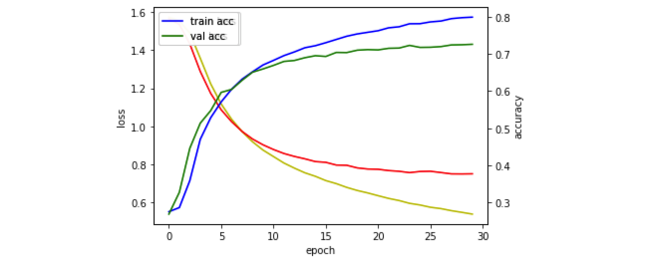
43903/43903 [==============================] - 1s 32us/sample - loss: 0.5399 - accuracy: 0.7997 - val_loss: 0.7513 - val_accuracy: 0.7265모델은 어제 가장 결과가 좋았던 모델을 가져와서
배치사이즈를 128에서 256으로
epoch를 20에서 30으로 늘려서 도출한 결과가 가장 좋아보여 이 모델을 활용했습니다.
결과 도출
# predict values
sample_submission = pd.read_csv("./sample_submission.csv")
pred = model2.predict_proba(test_padded)
sample_submission[['0','1','2','3','4']] = pred
sample_submission.to_csv('submission_13.csv', index = False, encoding = 'utf-8')
DACON 제출 결과

4일차의 최고기록 보다 더 나은 점수인 0.5122987567을 얻을 수 있었습니다.
여기서 batch size도 키우고 epoch도 늘려 도전한 점수가 더 좋은 것을 보고
베이스라인 코드에서 가장 좋았던 모델을 가지고 동일하게 batch size도 키우고 epoch도 늘려 학습해보면
어떤 결과가 나올까? 라는 의문이 들어 바로 시도해보았습니다.
전처리 방법은 4일차와 동일하니 4일차 게시물을 참고 바랍니다.
여러 모델 중에
기존에 Epoch 20, batch size 128을 Epoch 40, batch size 256 으로 변경하여 학습한 모델이
validation loss 와 validation accuracy를 봤을때 가장 좋은 것 같아 이 모델을 가지고 결과를 도출하고 제출해보았습니다.
model18 = tf.keras.Sequential([
tf.keras.layers.Embedding(vocab_size, embedding_dim, input_length=max_length),
tf.keras.layers.GlobalAveragePooling1D(),
tf.keras.layers.Dense(24, activation='relu'),
tf.keras.layers.Dropout(0.1),
tf.keras.layers.Dense(5, activation='softmax')
])
# compile model
model18.compile(loss='sparse_categorical_crossentropy',
optimizer='adam',
metrics=['accuracy'])
# model summary
print(model18.summary())
# fit model
num_epochs = 40
history18 = model18.fit(train_padded, y_train,
epochs=num_epochs, batch_size=256,
validation_split=0.2)Model: "sequential_5"
_________________________________________________________________
Layer (type) Output Shape Param #
=================================================================
embedding_5 (Embedding) (None, 500, 16) 320000
_________________________________________________________________
global_average_pooling1d_5 ( (None, 16) 0
_________________________________________________________________
dense_10 (Dense) (None, 24) 408
_________________________________________________________________
dropout_5 (Dropout) (None, 24) 0
_________________________________________________________________
dense_11 (Dense) (None, 5) 125
=================================================================
Total params: 320,533
Trainable params: 320,533
Non-trainable params: 0
_________________________________________________________________
None
Train on 43903 samples, validate on 10976 samples
Epoch 1/40
43903/43903 [==============================] - 3s 70us/sample - loss: 1.5773 - accuracy: 0.2632 - val_loss: 1.5688 - val_accuracy: 0.2680
Epoch 2/40
43903/43903 [==============================] - 3s 58us/sample - loss: 1.5666 - accuracy: 0.2762 - val_loss: 1.5650 - val_accuracy: 0.2680
...
Epoch 39/40
43903/43903 [==============================] - 3s 58us/sample - loss: 0.5108 - accuracy: 0.8191 - val_loss: 0.7594 - val_accuracy: 0.7239
Epoch 40/40
43903/43903 [==============================] - 3s 58us/sample - loss: 0.5009 - accuracy: 0.8223 - val_loss: 0.7590 - val_accuracy: 0.7239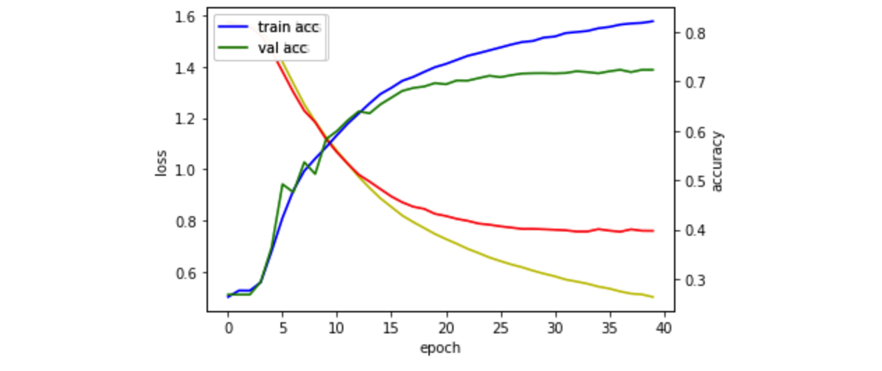
결과 도출
# predict values
sample_submission = pd.read_csv("./sample_submission.csv")
pred = model18.predict_proba(test_padded)
sample_submission[['0','1','2','3','4']] = pred
sample_submission.to_csv('submission_14.csv', index = False, encoding = 'utf-8')
DACON 제출 결과

음 여기서는 생각한 것과 다르게 4일차 최고 기록보다는 좋지 않은 결과를 얻었습니다.
베이스라인 전처리 방식을 잠시 미뤄두고
5일차인 오늘 처음 했던 전처리 방법에서 불용어를 좀 더 늘려서 시도해보기로 했습니다.
불용어를 늘리는 것은
stopwords_list = [ "a", "about", "above", "after", "again", "against", "all", "am", "an", "and", "any", "are", "as",
             "at", "be", "because", "been", "before", "being", "below", "between", "both", "but", "by", "could", "will",
             "did", "do", "does", "doing", "down", "during", "each", "few", "for", "from", "further", "had", "has",
             "have", "having", "he", "he'd", "he'll", "he's", "her", "here", "here's", "hers", "herself", "him", "himself",
             "his", "how", "how's", "i", "i'd", "i'll", "i'm", "i've", "if", "in", "into", "is", "it", "it's", "its", "itself",
             "let's", "me", "more", "most", "my", "myself", "nor", "of", "on", "once", "only", "or", "other", "ought", "our", "ours",
             "ourselves", "out", "over", "own", "same", "she", "she'd", "she'll", "she's", "should", "so", "some", "such", "than", "that",
             "that's", "the", "their", "theirs", "them", "themselves", "then", "there", "there's", "these", "they", "they'd", "they'll",
             "they're", "they've", "this", "those", "through", "to", "too", "under", "until", "up", "very", "was", "we", "we'd", "we'll",
             "we're", "we've", "were", "what", "what's", "when", "when's", "where", "where's", "which", "while", "who", "who's", "whom",
             "why", "why's", "with", "would", "you", "you'd", "you'll", "you're", "you've", "your", "yours", "yourself", "yourselves" ]
from nltk.corpus import stopwords
stopwords_list = stopwords_list + stopwords.words('english')baseline 코드에서 제공된 불용어와 nltk 라이브러리에서 제공해주는 불용어를 합한 데이터를 활용했습니다.
이렇게 만든 X_train 에 포함되어있는 유니크한 토큰의 개수는
불용어를 늘리기 전의 16,503개 보다 적은 16,478개 였습니다.
y_train = np.array([x for x in train_dataset['author']])새로 전처리 하는김에 Label 값도 One-Hot 인코딩하지 않고 그대로 사용했습니다.
import matplotlib.pyplot as plt
print("최대 길이 :" , max(len(l) for l in X_train))
print("평균 길이 : ", sum(map(len, X_train))/ len(X_train))
plt.hist([len(s) for s in X_train_vec], bins=50)
plt.xlabel('length of Data')
plt.ylabel('number of Data')
plt.show()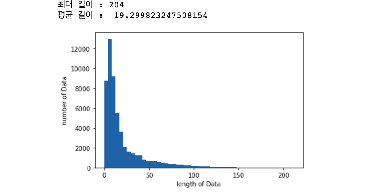
이렇게 만들어진 데이터의 최대 길이는 204, 평균 길이는 19였습니다.
#파라미터 설정
vocab_size = 16478
embedding_dim = 16
max_length = 204
padding_type='post'
이렇게 얻은 값들을 파라미터로 설정하였습니다.
위와 동일하게 데이터를 sequence로 변환해주고 padding 해 주었습니다.
model22 = tf.keras.Sequential([
    tf.keras.layers.Embedding(vocab_size, embedding_dim, input_length=max_length),
    tf.keras.layers.GlobalAveragePooling1D(),
    tf.keras.layers.Dense(24, activation='relu'),
    tf.keras.layers.Dropout(0.1),
    tf.keras.layers.Dense(5, activation='softmax')
])

# compile model
model22.compile(loss='sparse_categorical_crossentropy',
              optimizer='adam',
              metrics=['accuracy'])

# model summary
print(model22.summary())

# fit model
num_epochs = 30
history22 = model22.fit(train_padded, y_train,
                    epochs=num_epochs, batch_size=256,
                    validation_split=0.2)
Model: "sequential_10"
_________________________________________________________________
Layer (type) Output Shape Param #
=================================================================
embedding_10 (Embedding) (None, 204, 16) 263648
_________________________________________________________________
global_average_pooling1d_10 (None, 16) 0
_________________________________________________________________
dense_20 (Dense) (None, 24) 408
_________________________________________________________________
dropout_10 (Dropout) (None, 24) 0
_________________________________________________________________
dense_21 (Dense) (None, 5) 125
=================================================================
Total params: 264,181
Trainable params: 264,181
Non-trainable params: 0
_________________________________________________________________
None
Train on 43903 samples, validate on 10976 samples
Epoch 1/30
43903/43903 [==============================] - 2s 45us/sample - loss: 1.5781 - accuracy: 0.2637 - val_loss: 1.5658 - val_accuracy: 0.2680
Epoch 2/30
43903/43903 [==============================] - 1s 32us/sample - loss: 1.5588 - accuracy: 0.2789 - val_loss: 1.5481 - val_accuracy: 0.2695
...
Epoch 29/30
43903/43903 [==============================] - 1s 32us/sample - loss: 0.5477 - accuracy: 0.7980 - val_loss: 0.7324 - val_accuracy: 0.7332
Epoch 30/30
43903/43903 [==============================] - 1s 32us/sample - loss: 0.5432 - accuracy: 0.8010 - val_loss: 0.7317 - val_accuracy: 0.7316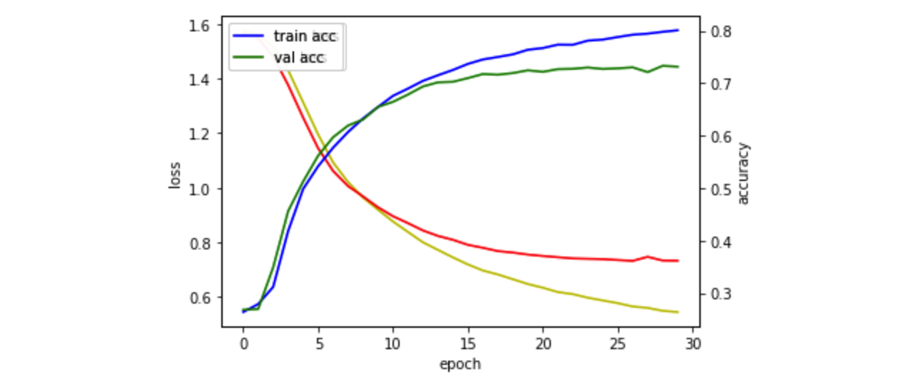
여러 파라미터들 중 위의 모델이 가장 좋아보여 결과를 도출하고 제출해보았습니다.
결과 도출
# predict values
sample_submission = pd.read_csv("./sample_submission.csv")
pred = model22.predict_proba(test_padded)
sample_submission[['0','1','2','3','4']] = pred
sample_submission.to_csv('submission_15.csv', index = False, encoding = 'utf-8')
DACON 제출 결과

오! 오늘도 최고기록을 경신했습니다! 0.4794888819!
금융문자 분석 경진대회 때는 이미 정확도가 90% 로 나와서 조금씩 올리기 너무 힘들었는데
이번에는 예측해야하는 클래스 수가 많아서 그런지
BERT와 같은 pre-trained 모델 사용이 불가해서 그런지 매일매일 최고기록을 경신하는 재미로 하고 있습니다.
불용어처리에 좀 더 신경쓰고 어간 추출을 진행한 전처리가 확실히 더 좋은 결과를 내는 것을 알 수 있었습니다.
내일은 표제어 추출을 전처리 과정에 넣어 시도해보려합니다.
그럼 읽어주셔서 감사합니다.
'DACON > 소설 작가 분류 AI 경진대회' 카테고리의 다른 글
| [DACON] 소설 작가 분류 AI 경진대회 N일차! (0) | 2020.11.05 |
|---|---|
| [DACON] 소설 작가 분류 AI 경진대회 6일차! (0) | 2020.11.04 |
| [DACON] 소설 작가 분류 AI 경진대회 4일차! (0) | 2020.11.02 |
| [DACON] 소설 작가 분류 AI 경진대회 1, 2, 3일차! (0) | 2020.11.01 |
| [DACON] 소설 작가 분류 AI 경진대회 도전! (0) | 2020.10.31 |


